Introduction and Warm Up Algebra
Bren Calculus Workshop
Carmen Galaz García, Ph.D.
Bren School of Environmental Science & Management
Last updated: Sep 17, 2025
Materials have been adapted and expanded from Nathaniel Grimes work for the Bren Calculus Workshop.
Workshop Objectives
Shake off the math dust
Equip students with the math skills to succeed in all Bren Courses
Explore how valuable math is to environmental science
Build a collaborative environment, crucial for success at Bren
About me
Carmen Galaz García (she/her)
Assistant Teaching Professor @ Bren
Before:
Data Scienist @ NCEAS
Ph.D. in Mathematics @ UCSB
Teaching & Research
Python courses and Capstone Projects for Masters in Environmental Data Science (MEDS)
Supporting math and data science across Bren!
NCEAS/TNC collaboration for invasive iceplant mapping analyzing remotely sensed images
Student Expectations
We expect all team students will:
Support and encourage all classmates
Be open to learning from each other
Bring a collaborative attitude and communicate respectfully
See opportunities to share kownledge as a chance to deepend understanding
Complete all in-class assessments
Logistics
No food in BH 1414
If you are feeling sick: stay home and take care of yourself! Please mask up if you are not feeling 100%.
Math in Environmental Science
Share with the person next to you:
What has been your life or professional experience with math? Best friend ever, mortal enemy, or something in between?
How do you see math being relevant to solving environmental problems?
Math is an important tool in environmental science
Math helps us investigate the world and communicate our findings
Used by scientists to find evidence
Can be used to quantify relations, trends, and changes
Mathematical models can help us understand complex systems
Must be used responsibly and with awareness of potential biases and limitations
Helps us support arguments that can transform policy and actions
We need to understand the math to make decisions on it!
Math at Bren
ESM 201: Ecology of Managed Ecosystems
Lotka-Volterra Models \[
\begin{align}
\frac{dN_1}{dt}&=r_1N_1\left(\frac{K_1-N_1-\alpha N_2}{K_1}\right)\\
\frac{dN_2}{dt}&=r_2N_2\left(\frac{K_2-N_2-\beta N_1}{K_2}\right)
\end{align}
\]
ESM 222: Pollution Risk Management
Groundwater transport of absorbed contaminant \[
\frac{\partial C}{\partial t}=\left(\frac{D}{R}\frac{\partial^2t}{\partial x^2}\right)-\left(\frac{v}{R}\frac{\partial C}{\partial x}\right)-\frac{k}{R}C
\]
Rules of Algebra
Never change an equation. Instead, we rewrite them into more useful forms
Manipulate BOTH sides of an equation with the SAME PROCEDURE.
Always add/substract/multiply/divide by the same number on both sides. More generally, always apply the same function to both sides of the equation.
Order of Operations, a.k.a. PEDMAS: (P)aranthesis (E)xponents (D)ivide (M)ultiply (A)dd (S)ubtract
PEDMAS important for what order to manipulate equations
\[
z = 4*(y-4)+(x+1)^2
\]
If we are given the values of \(x=-3\) and \(y=2\) , what would be the value of \(z\) ?
✏️ Take a minute to solve this individually.
PEDMAS important for what order to manipulate equations
If we are given the values of \(x=-3\) and \(y=2\) , what would be the value of \(z\) ?
💡 Let’s see a solution!
\[
\begin{align}
z &= 4*(y-4)+(x+1)^2 \\
&= 4*(2-4)+(-3+1)^2 \\
&= 4*(-2)+(-2)^2 \\
&= -8 + 4 \\
&= -4.
\end{align}
\]
Often times we want flexible equations
Prices are important in economics, but not always available for environmental goods.
How do we get prices if we know quantity?
\[
\require{cancel}
\begin{aligned}
Q&=\frac{(400-P)}{80} &\text{Isolate P in terms of Q} \\
\end{aligned}
\]
✏️ Take a minute to solve this individually.
Often times we want flexible equations
💡 Let’s see a solution!
Prices are important in economics, but not always available for environmental goods.
How do we get prices if we know quantity?
\[
\require{cancel}
\begin{aligned}
Q&=\frac{(400-P)}{80} &\text{Isolate P in terms of Q} \\
80Q&=\frac{(400-P)\cancel{80}}{\cancel{80}} &\text{ Multiply both sides by 80} \\
80Q-400&=\cancel{400}-\cancel{400} -P &\text{ Subtract both sides by 400} \\
-1(80Q-400)&=-P(-1) &\text{Multiply both sides by -1} \\
400-80Q&=P &\text{Flip terms for simplicity}
\end{aligned}
\]
It can be easy to make mistakes while doing algebra. Practice makes perfect!
Solve all in terms of \(x\)
\(3x+2=10x-12\)
\(4-3(2x+1)=8-\frac{3x}{2}\)
\(3(x+7a)-5=b+2(c-4x)\)
✏️ Take a minute to solve these individually.
It can be easy to make mistakes while doing algebra. Practice makes perfect!
💡 Let’s see a solution!
Solve all in terms of \(x\)
\(4-3(2x+1)=8-\frac{3x}{2}\)
It can be easy to make mistakes while doing algebra. Practice makes perfect!
💡 Let’s see a solution!
Solve all in terms of \(x\)
\(3(x+7a)-5=b+2(c-4x)\)
Practice Solutions
\[
\small
\begin{aligned}
3x+2&=10x-12 \\
3x+2+12&=10x-12(+12) \\
3x-3x+14&=10x-3x \\
14&=7x \\
x&=2
\end{aligned}
\]
\[
\small
\begin{aligned}
4-3(2x+1)&=8-\frac{3x}{2}\\
4-3-6x&=8-\frac{3x}{2} \\
1-6x&=8-\frac{3x}{2} \\
2-12x&=16-3x \\
-9x&=14 \\
x&=\frac{-14}{9}\\
\end{aligned}
\]
\[
\small
\begin{aligned}
3(x+7a)-5&=b+2(c-4x)\\
3x+21a-5&=b+2c-8x \\
11x+21a-5&=b+2c \\
11x&=5+b+2c-21a\\
x&=\frac{5+b+2c-21a}{11}
\end{aligned}
\]
Exponents make algebra more interesting!
Example
The expression \(x^3\) means \(x\) multiplied by itself 3 times: \[x^3=x * x * x\]
More generally, \[x^n = x \text{ to the power of } n.\]
Intuitively, the exponent \(n\) tells us how many times to multiply the basis \(x\) by itself:
\[x^n = \underbrace{x * x * ... * x}_{n \text{ times}}\]
But the exponent can be any (real) number, not only integers!
What are exponents good for?
They can describe really big numbers
Diameter of the Milky Way = 1,000,000,000,000,000,000,000 meters = \[10^{21} \text{ m}\]
And also really small numbers
Diameter of a human red blood cell = 0.0000000001 meters = \[10^{-10} \text{ m}\]
This way, we can use exponents to describe exponential growth and decay. Many environmental variables behave in this way.
Rules and properties of exponents (1)
Product rule:
Quotient rule:
Any non-negative \(x\) to the power of 0 equals 1:
Negative exponent means divide:
Fractional exponent means take the \(n\) -th root:
Rules and properties of exponents (2)
Power of a power means multiply the exponents:
Exponents get distributed over products:
And exponents get distributed over divisions:
If \(a\) is the \(n\) -th root of \(x\) , then \(a\) to the \(n\) equals \(x\) :
Rules and properties of exponents (1)
Product rule: \(x^a * x^b = x^{a+b}\)
Quotient rule: \(\frac{x^a}{x^b} = x^{a-b}, \ \ \text{for } x \neq 0\)
Any non-negative \(x\) to the power of 0 equals 1: \(x^0 = 1, \ \ \text{for } x \neq 0\)
Negative exponent means divide: \(x^{-a} = \frac{1}{x^a}, \ \ \text{for } x \neq 0\)
Fractional exponent means take the \(n\) -th root: \(x^{\frac{1}{n}} = \sqrt[n]{x}\)
Rules and properties of exponents (2)
Power of a power means multiply the exponents: \((x^a)^b = x^{ab}\)
Exponents get distributed over products: \((xy)^a = x^a y^a\)
And exponents get distributed over divisions: \(\left( \frac{x}{y} \right)^a = \frac{x^a}{y^a}\)
If \(a\) is the \(n\) -th root of \(x\) , then \(a\) to the \(n\) equals \(x\) :
\[
a = \sqrt[n]{x} \Rightarrow a^n = x
\]
Rules and properties of exponents
\[
\begin{array}{|l|l|}
\hline
\textbf{Rule} & \textbf{Expression} \\
\hline
\text{Product Rule} & x^{a} \cdot x^{b} = x^{a+b} \\
\hline
\text{Quotient Rule} & \frac{x^{a}}{x^{b}} = x^{a-b}, \quad x \neq 0 \\
\hline
\text{Zero Exponent} & x^{0} = 1, \quad x \neq 0 \\
\hline
\text{Negative Exponent} & x^{-a} = \frac{1}{x^{a}}, \quad x \neq 0 \\
\hline
\text{Fractional Exponent} & x^{\frac{1}{n}} = \sqrt[n]{x} \\
\hline
\text{Power of a Power} & (x^{a})^{b} = x^{ab} \\
\hline
\text{Power of a Product} & (xy)^{a} = x^{a}y^{a} \\
\hline
\text{Power of a Quotient} & \left(\frac{x}{y}\right)^{a} = \frac{x^{a}}{y^{a}} \\
\hline
\text{$n$-th Root Definition} & a = \sqrt[n]{x} \quad \Rightarrow \quad a^{n} = x \\
\hline
\end{array}
\]
Exponents practice
✏️ Simplify the following.
\(\frac{6^5}{6^3}\)
\((x^2y)^4\)
\(\frac{x^5y^6}{xy^2}\)
\(\frac{24x^6}{12x^{-8}}\)
\[
\begin{array}{|l|l|}
\hline
\textbf{Rule} & \textbf{Expression} \\
\hline
\text{Product Rule} & x^{a} \cdot x^{b} = x^{a+b} \\
\hline
\text{Quotient Rule} & \frac{x^{a}}{x^{b}} = x^{a-b}, \quad x \neq 0 \\
\hline
\text{Zero Exponent} & x^{0} = 1, \quad x \neq 0 \\
\hline
\text{Negative Exponent} & x^{-a} = \frac{1}{x^{a}}, \quad x \neq 0 \\
\hline
\text{Fractional Exponent} & x^{\frac{1}{n}} = \sqrt[n]{x} \\
\hline
\text{Power of a Power} & (x^{a})^{b} = x^{ab} \\
\hline
\text{Power of a Product} & (xy)^{a} = x^{a}y^{a} \\
\hline
\text{Power of a Quotient} & \left(\frac{x}{y}\right)^{a} = \frac{x^{a}}{y^{a}} \\
\hline
\text{$n$-th Root Definition} & a = \sqrt[n]{x} \quad \Rightarrow \quad a^{n} = x \\
\hline
\end{array}
\]
Exponents practice
✏️ Let’s see a solution.
\(\frac{6^5}{6^3} = 6^{5-3} = 6^2\)
\((x^2y)^4 = (x^2)^4*y^2 = x^8y^2\)
\(\frac{x^5y^6}{xy^2} = \frac{x^5}{x}*\frac{y^6}{y^2} = x^{5-1}*y^{6-2} = x^4y^4 = (xy)^4\)
\(\frac{24x^6}{12x^{-8}} = 2x^6x^{(-(-8))}=2x^6x^8 = 2x^{6+8} = 2x^{14}\)
Polynomials describe more complex relationships through exponents
A polynomial is a function of the form: \[
\large
\begin{align}
a_nx^n+a_{n-1}x^{n-1}+...+a_1x+a_0
\end{align}
\]
\(x\) is the variable \(a_i\) are constants (fixed numbers) that are called the coefficients of the polynomialeach \(a_ix^i\) is called a term of the polynomial,
\(n\) is called the degree of the polynomial, this is the largest exponent in the polynomial.
Example:
Polynomials often represent real world data better than a linear function.
Fundamental Theorem of Algebra
A zero , root , or solution for a polynomial is a value of \(x\) that makes the polynomial equal to zero.
Fundamental Theorem of Algebra
A polynomial \[
a_nx^n+a_{n-1}x^{n-1}+...+a_1x+a_0
\]
of degree \(n\) has exactly \(n\) roots \(r_1, \ldots, r_n\) and it can be refactored as
\[
c(x-r_1) ... (x-r_n)
\]
The numbers \(c\) and \(r_1, \ldots, r_n\) may be complex!
Example: linear equation
A linear equation is just a 1st degree polynomial. How many solutions does it have?
\[
3x+2=10x-12
\]
This can be rewritten as:
\[
x - 2 = 0.
\]
So \(r_1 = 2\) is the root. There is a single root because the degree is 1.
Finding the roots of \(n\) -th degree polynomials is much harder - we will let computers do it for us.
Let’s zoom in on 2nd degree polynomials
Example: second degree polynomial
What happens if \(x=4\) or \(x=-3\) in \(x^2-x-12\) ?
This means 4 and 3 are roots of the polynomial \(x^2-x-12\) .
The only way to get \(x^2-x-12=0\) is for \(x\) to either be 4 or -3.
We can rewrite \[x^2-x-12 = (x-4)(x+3).\]
Verify the factorization on the right.
Quadratic Formula solves 2nd degree polynomials
For any second degree polynomial
\[
ax^2+bx+c=0
\]
The roots to can be found using the quadratic formula:
\[
x=\frac{-b\pm\sqrt{b^2-4ac}}{2a}
\]
Example:
Let’s use the quadratic formula to find the solutions to \(x^2-x-12=0\) .
Identify which numbers you should plug into which variable of the quadratic formula (e.g. a,b,c)
\[
4x^2+x-14=0
\]
Identify which numbers you should plug into which variable of the quadratic formula (e.g. a,b,c)
\[
256-\sqrt{44}x^2+.23x=10
\]
What happens if \(b^2-4ac\) is negative in the quadratic formula?
Expand \((3x-6)(2x+1)\)
Solutions
\[
4x^2+x-14=0
\]
\[
\begin{aligned}
a=4 \\
b=1 \\
c=-14
\end{aligned}
\]
Solutions
\[
256-\sqrt{44} x^2+.23x=10
\]
\[
\begin{aligned}
a=\sqrt{44} \\
b=.23 \\
c=246
\end{aligned}
\]
This will probably be a nasty calculation, but that is what computers are for. The order does not matter, only that the \(a\) corresponds to the square term, the \(b\) to the 1st degree term, and the \(c\) to the constant.
Solutions
What happens if \(b^2-4ac\) is negative in the quadratic formula
There are no real solutions, but complex (imaginary) solutions. This means numbers of the form \(a+ib\) where \(i = \sqrt{-1}\) . These can still be useful - but that’s for another class!
Solutions
Expand \((3x-6)(2x+1)\)
\[
\begin{align}
(3x-6)(2x+1) \\
6x^2+3x-12x-6 \\
6x^2-9x-6
\end{align}
\]
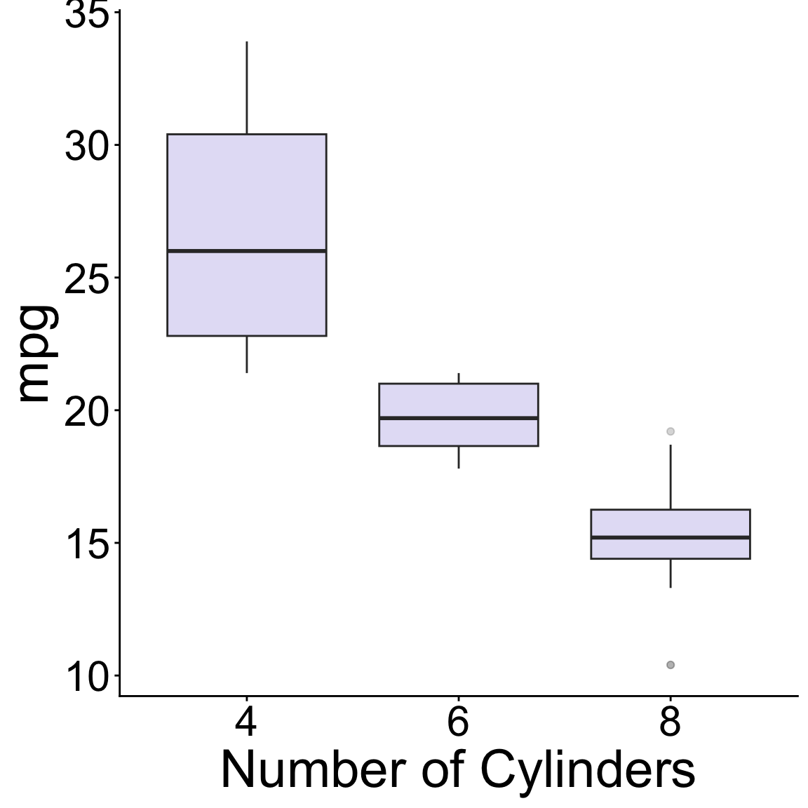
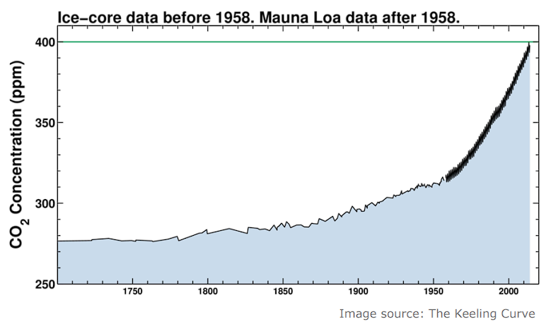
Graphs bring visual connection to math and data
Which looks better and is easier to understand?
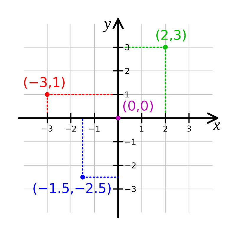
The \(xy\) coordinate system
Graphs move in a 2-dimensional plane with a coordinate system using two axes:
Axes units must be defined depending on the application.
We use pairs of numbers to place data:
A point on the \(xy\) plane with coordinates \((a,b)\) means the point is located at \(a\) on the \(x\) -axis and at \(b\) on the \(y\) -axis.
Where would (2,-1) go on the graph?
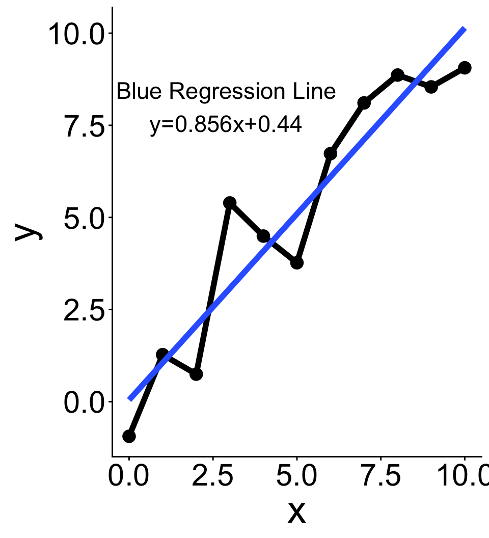
We can join series of points to make graphs
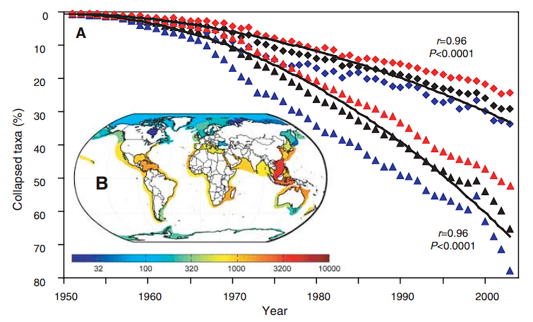
Real life example: seafood depletion
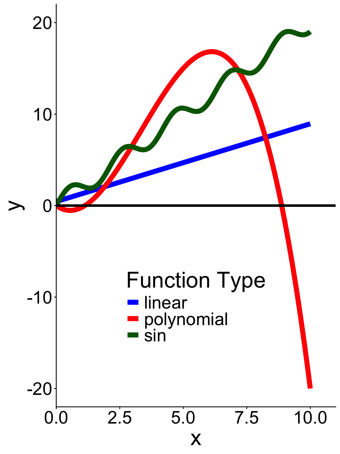
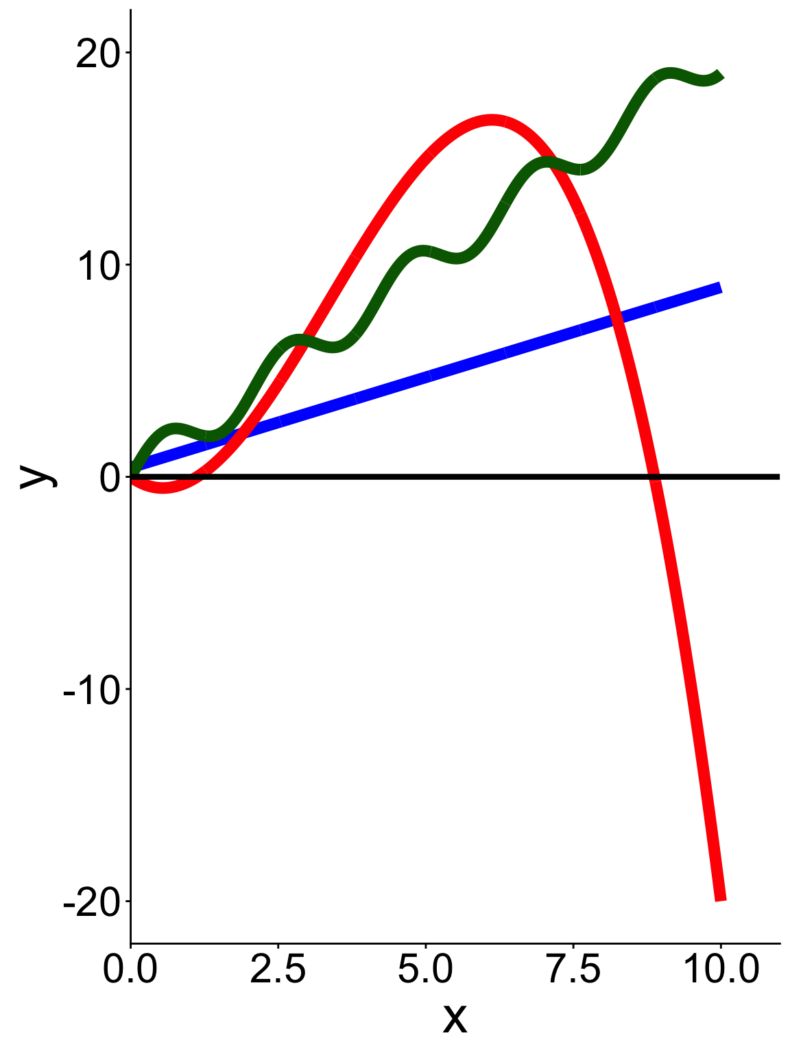
Functions on a single variable and a single output can be graphed
\(\color{green}{y=sin(3x)+2x}\)
\(\color{red}{y=0.5x^3+x^2-5x}\)
\(\color{blue}{y=0.85x+0.44}\)
Two key ingredients to graphs
Intercepts
\(x\) -intercept
Where does the graph intersect the \(x\) -axis?
In other words, for what values of \(x\) do we have \((x,0)\) be part of the graph?
\(y\) -intercept
Where does the graph intersect the \(y\) -axis?
In other words, for what value of \(y\) do we have \((0,y)\) be part of the graph?
What are the intercepts of the polynomial function in red?
Linear functions: slope-intercept form
Easiest model to describe linear relationship between two variables!
\[
\huge
\begin{align}
\underbrace{y}_{\text{output}}=\overbrace{m}^{\text{Slope}}\underbrace{x}_{\text{input}}+\overbrace{b}^{\text{$y$ intercept}}
\end{align}
\]
The slope tells us how quickly is the line changing.
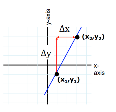
How to calculate the slope?
Slope =
vertical change per unit of horizontal change.
\[
m=\frac{\Delta y}{\Delta x}=\frac{y_2-y_1}{x_2-x_1}
\]
Horizontal Slope: \(m=0\)
Vertical Slope: \(m\) is undefined
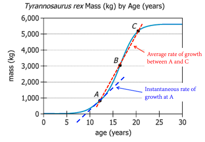
Slope represents rate of change
Slope can be average or instantaneous
Rise over run can always be used to find average rate of change between two parts of a graph
Instantaneous rate of change leads us to ✨calculus✨.
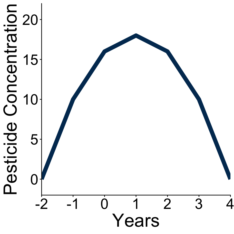
Your team measured the concentrations of pesticides in a lake exposed to agricultural runoff. You have the following equation describing the total amount of pesticides in the lake if runoff is stopped from the farm by a new policy incentive reducing pesticides use:
\[
\begin{aligned}
&y=(8-2t)(t+2) \\
&\text{Where } y \text{ is pesticde concentration in ppb} \\
&\text{and } t \text{ is time in years}.
\end{aligned}
\]
Work with your team to
first discuss conceptually how you would solve all the following tasks, do not write anything!
second work out with pen and paper the solutions to verify the ideas you discussed.
What kind of equation is this? Would it be useful to write it in another form?
How long will it take for the pesticide concentration in the lake to reach zero? Since the equation is a polynomial describe why one solution is more applicable than the other.
Present your findings (choose between a graph or table).
What is the average change in concentration from year 0 to year 4?
Explain to your client why concentrations might behave the way they were modeled.
Solution 1
Let’s expand out the equation so it becomes easier to graph.
\[
\begin{aligned}
y&=(-2t+8)(t+2) \\
y&=\overbrace{-2t^2}^{\text{First}}-\overbrace{4t}^{\text{Outside}}+\overbrace{8t}^{\text{Inside}}+\overbrace{16}^{\text{Last}}\\
y&=-2t^2+4t+16
\end{aligned}
\]
Solution 2
Use the Quadratic Formula
\[
\begin{aligned}
0&=-2t^2+4t+16 \\
0&=\frac{-4\pm\sqrt{4^2-4(-2)(16)}}{2(-2)}\\
0&=\frac{-4\pm\sqrt{16+128}}{-4} \\
&t=4\text{, } t=-2
\end{aligned}
\]
\[
\begin{aligned}
2t-8=0 \\
t=\frac{8}{2}\\
t=4
\end{aligned}
\]
Solution 3
= seq (- 2 ,4 )= - 2 * t^ 2 + 4 * t+ 16 <- data.frame (t= t,y= y)<- df %>% ggplot (aes (x= t,y= y))+ geom_line (color= "#003660" ,linewidth= 3 )+ labs (x= "Years" ,y= "Pesticide Concentration" )+ scale_x_continuous (expand = c (0 , 0 )) + scale_y_continuous (expand = c (0 , 0 ),limits = c (- 2 ,22 ))+ theme_classic ()+ theme (text = element_text (size = 28 ))
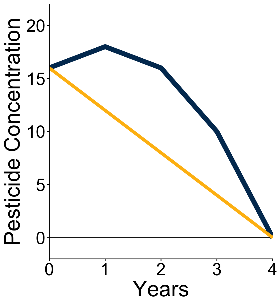
Solution 4
<- df %>% filter (t>= 0 ) %>% ggplot (aes (x= t,y= y))+ geom_line (color= "#003660" ,linewidth= 3 )+ labs (x= "Years" ,y= "Pesticide Concentration" )+ scale_x_continuous (expand = c (0 , 0 )) + scale_y_continuous (expand = c (0 , 0 ),limits= c (- 2 ,22 ))+ geom_hline (yintercept = 0 )+ annotate ("segment" ,x= 0 ,xend= 4 ,y= 16 ,yend= 0 ,color= "#FEBC11" ,linewidth= 2 )+ theme_classic ()+ theme (text = element_text (size = 28 ))
Use rise over run:
\[
\frac{\Delta y}{\Delta x}=\frac{0-16}{4-0}=-4
\]
Pesticides are removed from the lake at an average rate of 4 ppb per year.
Solution 5
Pesticide concentrations might initially increase in the lake from residual particles in the soil being washed into the lake. Then a mixture microbial activity and other chemical process reduce the pesticides to more inert components.
(You will learn the actual answer in ESM 202: Environmental Biogeochemistry)