Solutions: Algebra and Graphing Problem Set

Answer the following questions to the best of your ability. Attempt exercises on your own first to make sure you fully understand the concepts. Feel free to work with anyone in the cohort after giving the problems a try!

Algebra basics

Describe how solving for the roots of equations (the values of $x$ for which a function $f(x)$ satisfies $f(x)=0$) could be useful in environmental science. List at least one method to find roots of a certain kind of funciton.

Finding the roots of an equation could be useful to, for example, predict when the concentration of pollutants reaches zero, or when does the cost and benefits of a program balance. Any answers in that direction could be good.

One method for finding roots would be to use the quadratic formula if the function is a quadratic function..

Expand the following expressions:

\[ \begin{align} (x+2)(3x-4) &=& 3x^2-4x+6x-8 \\ &=& 3x^2+2x-8 \end{align} \]

\[ \begin{align} (x^2-2y)(x+y^3) = x^3+x^2y^3-2yx-2y^4 \end{align} \]

Solve for $x$ in the following equations:

\[ \begin{align} 2x-4=&3x+12 \\ 2x&=3x+16 &\text{Add 4 to both sides}\\ -x&=16 &\text{Subtract $3x$ from both sides}\\ x&=16 \end{align} \]

b. \[ \begin{align} -6ax+2b&=x-5c \\ -6ax&=x-5c-2b &\text{Subtract $2b$ from both sides} \\ -6ax-x&=-5c-2b &\text{Subtract $x$} \\ x(-6a-1)&=-5c-2b &\text{Factor out $x$}\\ x&=\frac{-5c-2b}{(-6a-1)} \end{align} \]

c. \[ \begin{align} 2x^2+3x-4&=0 \\ \frac{-(3)\pm\sqrt{3^2-4(2*-4)}}{2(2)}&=0 \\ x_1=\frac{-3+\sqrt{41}}{4}& &x_2=\frac{-3-\sqrt{41}}{4} \\ x_1\approx0.85 & &x_2\approx-2.35 \end{align} \]

d. \[ \begin{align} x^2+2x-5&=0 \\ \frac{-(-2)\pm\sqrt{2^2-4(1*-5)}}{2(1)}&=0 \\ x_1=\frac{2+\sqrt{24}}{2}& &x_2=\frac{2-\sqrt{24}}{2} \\ x_1\approx3.45 & &x_2\approx-1.45 \end{align} \]

Story Problems

Representative Concentration Pathways (RCP) are climate change scenarios that project future greenhouse gas concentrations in 2100. A new RCP projection indicates that carbon concentrations in the atmosphere will plateau at around 600 ppm. Today’s atmospheric carbon concentration sits at 416 ppm.
1. If the United States continues to emit proportionally the same amount of carbon (14%), how much carbon will the US emit in 2100 under RCP 4.5? Use the conversion 1 ppm=2.13 gigaton to give your answer in gigatons.

Since the fraction of US carbon emissions will remain constant at 14% we can calculate that the US will emit 14% of the 600 ppm in 2100:

\[ \begin{align} 600 * 0.14 &=& 84 \text{ ppm}\\ &=& 84* 2.13 \text{ gigaton}\\ &=& 178.92 \text{ gigaton} \end{align} \]

Let’s say the US decides to pursue an ambitious policy to extract their contribution of carbon from the air. Climatologists model that this policy would have a trajectory of $f(t)=\frac{-1}{8}t^2+6t+123.83$ where $t$ is each year and $f(t)$ is the amount of carbon released by the US. When will the United States eliminate their carbon footprint?

Based on the model of the scientists, we need to where the total amount of US carbon equals 0. In other words, we need to find when \[f(t) = \frac{1}{8}t^2+6t+123.83=0.\]

Because $f(t)$ is a second degree polynomial we can use the quadratic equation to find it’s roots:

\[ \begin{align} t &=& \frac{-6\pm\sqrt{6^2-4(\frac{-1}{8}*123.83)}}{\frac{-2}{8}} \\ t &\approx& 63.581 \text{ years} \end{align} \]

We are only concerned about the postive year amounts.

Graphs

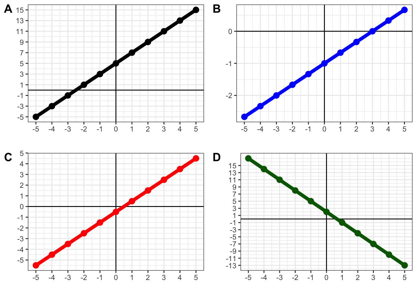
Find the slope and $y$-intercept of the following lines.

Show the code

x=seq(-5,5)

y=2*x+5

w=(1/3)*x-1

z=x-0.5

u=-3*x+2

p1<-ggplot()+
  geom_hline(yintercept=0)+
  geom_vline(xintercept = 0)+
  geom_point(aes(x=x,y=y),size=3,color="black")+
  geom_line(aes(x=x,y=y),size=2,color="black")+
  theme_bw()+
  theme(axis.line = element_blank())+
  scale_y_continuous(breaks=seq(-5,15,2))+
  scale_x_continuous(breaks=seq(-5,5,by=1))+
  labs(x="",y="")

p2<-ggplot()+
  geom_hline(yintercept=0)+
  geom_vline(xintercept = 0)+
  geom_point(aes(x=x,y=w),size=3,color="blue")+
  geom_line(aes(x=x,y=w),size=2,color="blue")+
  theme_bw()+
  theme(axis.line = element_blank())+
  scale_y_continuous(breaks=seq(-3,3,1))+
  scale_x_continuous(breaks=seq(-5,5,by=1))+
  labs(x="",y="")

p3<-ggplot()+
  geom_hline(yintercept=0)+
  geom_vline(xintercept = 0)+
  geom_point(aes(x=x,y=z),size=3,color="red")+
  geom_line(aes(x=x,y=z),size=2,color="red")+
  theme_bw()+
  theme(axis.line = element_blank())+
  scale_y_continuous(breaks=seq(-5,5,1))+
  scale_x_continuous(breaks=seq(-5,5,by=1))+
  labs(x="",y="")

p4<-ggplot()+
  geom_hline(yintercept=0)+
  geom_vline(xintercept = 0)+
  geom_point(aes(x=x,y=u),size=3,color="darkgreen")+
  geom_line(aes(x=x,y=u),size=2,color="darkgreen")+
  theme_bw()+
  theme(axis.line = element_blank())+
  scale_y_continuous(breaks=seq(-15,15,2))+
  scale_x_continuous(breaks=seq(-5,5,by=1))+
  labs(x="",y="")

cowplot::plot_grid(p1,p2,p3,p4,labels=c("A","B","C","D"))

The slope for graph A is 2 with a $y$-intercept of 5.

The slope for graph B is 1/3 with a $y$-intercept of -1

The for graph C is 1 with a $y$-intercept of -0.5

The slope for graph D is -3 with a $y$-intercept of 2

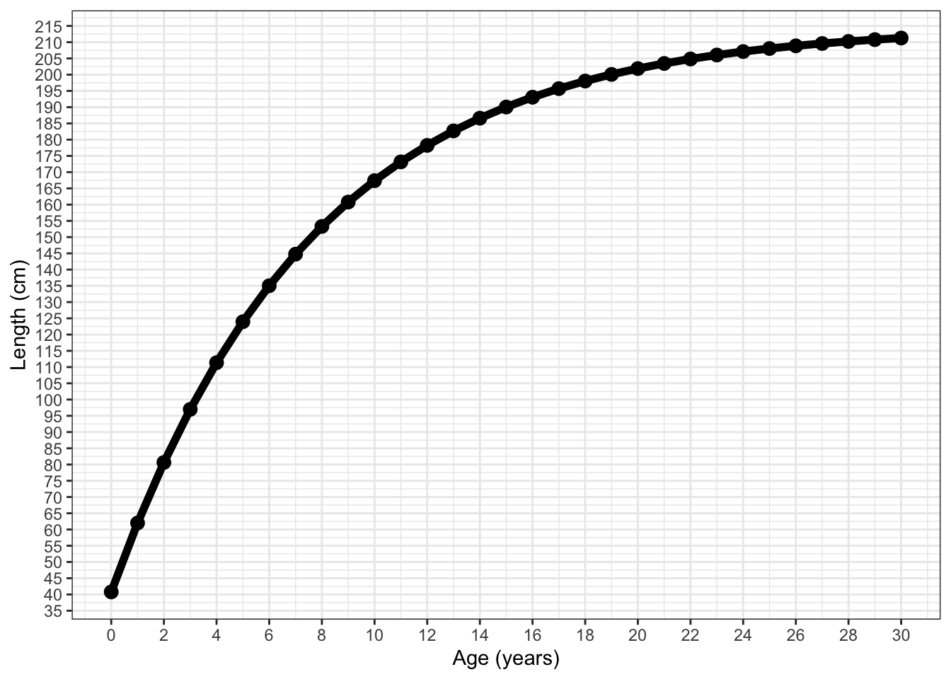
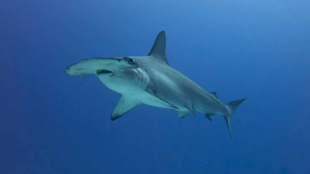
The growth of sharks can be modeled using von Bertalanffy curves. Scalloped hammerhead sharks in the Atlantic were found to have growth curves that follow the graph below.

Show the code

vb<-function(a,l,k,t0){
  l*(1-exp(-k*(a-t0)))
}

x=seq(0,30)

length=vb(x,214.8,.13,-1.62)

p1<-ggplot()+
  geom_point(aes(x=x,y=length),color="black",size=3)+
  geom_line(aes(x=x,y=length),color="black",size=2)+
  theme_bw()+
  scale_y_continuous(breaks=seq(35,215,5))+
  scale_x_continuous(breaks=seq(0,32,by=2))+
  labs(x="Age (years)",y="Length (cm)")

p1

What is the average slope from ages 0 to 8? From 20 to 30?

The average slope from ages 0 to 8 can be calcualted by: \[ slope = \frac{155-40}{8-0} = 14.375\]

The average slope from ages 0 to 8 can be calcualted by: \[ slope = \frac{210-200}{30-20} =1 \]

This tells us that the average rate of change for sharks between the ages of 0 to 8 was 14.375. For the ages, 20 to 30 the average change was 1.

What are the units of the average slopes and why would they change for a shark as they get older?

Slopes are in units of length over age, so the slope indicates the growth in centimeters every year. As animals get older, ther slow down their growth. Less energy is spent in growing and more invested in reproductive energy.

How would you find the instantaneous slope for a shark at age 12? What is the closest approximation you can make with this data and graph?

We would need to apply calculus to find the true answer, but we can approximate it reasonably well by finding the smallest possible difference between two points around age 12. In this case we can use $\frac{175-172}{13-12}$ to get an approximate instaneous rate of growth of 3 cm per year.

Picture of a scalloped hammerhead shark.