Bren Calculus Workshop – lecture-diffeq

Differential Equations and Numerical Calculus

Bren Calculus Workshop

Carmen Galaz García, Ph.D.

Bren School of Environmental Science & Management

Last updated: Sep 23, 2025

Materials have been adapted and expanded from Nathaniel Grimes work for the Bren Calculus Workshop.

Integral of the exponential function

Since $\frac{d}{dx}e^x = e^x$, we have that

\[ \large \int e^xdx=e^x+C \]

If the $x$ term gets more complex, we need integration by parts or substitution.

This can get complicated and ee will not cover it in the workshop.

Natural logs in integration

Since $\frac{d}{dx} \ln(x) = \frac{1}{x}$ we have that

\[ \large \int \frac{1}{x}=\ln x+C. \]

On the other hand, we have that

\[ \begin{align} \int \ln x&=x\ln x-x+C \end{align} \]

This is computed using integration by parts.

✏️ How would you check this second integral is correct?

Introduction to Differential Equations

What is a differential equation?

A differential equation is any equation which contains derivatives.

The goal of the differential equation is to find a function that satisfies the equation.

Ordinary differential equations (ODEs) are differential equations with ordinary derivatives (the ones we have been working with).

Sometimes functions have more than one variable and we can take partial derivatives with respect to each variable. Differential equations with partial derivatives are called partial differential equations (PDEs).

Example

What is a differential equation?

A differential equation is any equation which contains derivatives.

The goal of the differential equation is to find a function that satisfies the equation.

Ordinary differential equations (ODEs) are differential equations with ordinary derivatives (the ones we have been working with).

Example

The equation

\[ y' = y + x \]

is a differential equation in which we want to find a function $y(x)$ such that its derivative equals the function plus $x$.

✏️ Check that $y(x) = -x -1$ is a solution for this differential equation.

Differential equations help us understand changing environments

For some natural phenomena it can be easier to describe them in terms of derivatives than give an explicit function.

Example

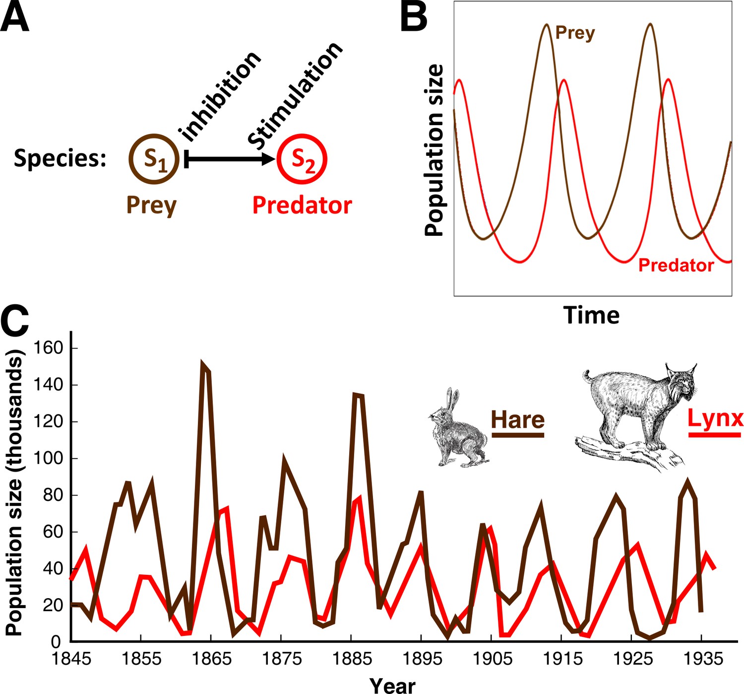
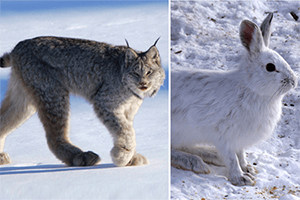
Lotka-Volterra models to describe preadtor prey dynamics: \[ \begin{align} \frac{dN_1}{dt}&=r_1N_1\left(\frac{K_1-N_1-\alpha N_2}{K_1}\right)\\ \frac{dN_2}{dt}&=r_2N_2\left(\frac{K_2-N_2-\beta N_1}{K_2}\right) \end{align} \]

where $N_1, N_2$ are the popylation of prey and preadtor respectively.

Differential equations are systems in motion

Differential equations relate a quantity to its rate of change.
By specifying how something changes, we are describing a process over time.
We are finding whole trajectories or behaviors over time.

Where will you run into ODEs?

ESM 201: Ecology of Managed Ecosystems

Lotka-Volterra Models \[ \begin{align} \frac{dN_1}{dt}&=r_1N_1\left(\frac{K_1-N_1-\alpha N_2}{K_1}\right)\\ \frac{dN_2}{dt}&=r_2N_2\left(\frac{K_2-N_2-\beta N_1}{K_2}\right) \end{align} \]

ESM 222: Pollution Risk Management

Groundwater transport of absorbed contaminant \[ \frac{\partial C}{\partial t}=\left(\frac{D}{R}\frac{\partial^2t}{\partial x^2}\right)-\left(\frac{v}{R}\frac{\partial C}{\partial x}\right)-\frac{k}{R}C \]

Solving Differential Equations

Separation of variables

A first-order ODE of the form $\frac{dy}{dx} = f(x)g(y)$ can be solved in the following steps:

✏️ Solve for $y$ in $\frac{dy}{dx}=4y$

Separation of variables

A first-order ODE of the form $\frac{dy}{dx} = f(x)g(y)$ can be solved in the following steps:

Move like terms to the same side, including differentials $dx\text{ and } dy$. This is a convenient shorthand for more involved calculus steps.
Apply the integral to both sides.
Rearrange equations to isolate in terms of dependent variable.
Use initial conditions (if given) to find $C$ values.
Evaluate the bounds if definite intervals are given.

✏️ Solve for $y$ in $\frac{dy}{dx}=4y$

\[ \begin{align} \frac{dy}{4y}& =dx \\ \int\frac{dy}{4y}&=\int dx\\ \frac{1}{4}\ln y&=x+C_1 \\ \ln y&=4x+C_2\\ y&=e^{4x+C_2} \\ y&=e^{C_2}e^{4x} \\ y&=Ce^{4x} \end{align} \]

Team Assessment

Verify that \[\int \frac{1}{ax+b} dx = \frac{\ln(ax+b)}{a}.\]

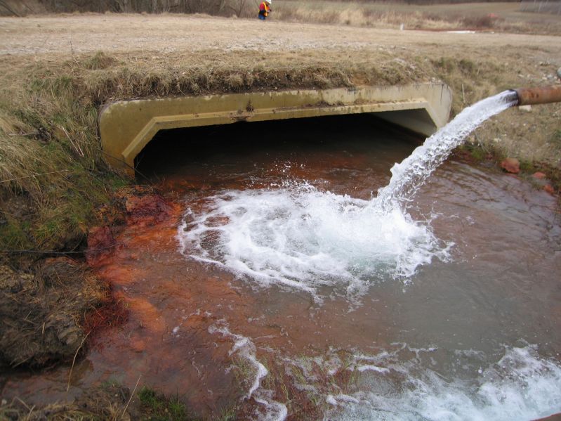
An oil spill off the coast of Santa Barbara is spreading rapidly. Previous spills and an analysis of the current data indicate that the oil is spreading at a daily rate of:

\[ \frac{dA}{dt}=-0.001A+60, \]

where $A$ is the area of the oil spill in $km^2$ and $t$ is the time in days.

Find an equation that models the spread of oil in total area. Hint: exercise 1.
After the first day the oil has spread to 25 $km^2$. What steps would you take to find when will the oil spill cover all of the Santa Barbara Channel (~5850 $km^2$)? You don’t need to compute it, just come up with a solid plan.

Solution 2.a.

We are given the differential equation:

\[ \frac{dA}{dt} = -0.001 A + 60 \]

Step 1: Rearrange for separation of variables

\[ \frac{dA}{dt} = 60 - 0.001 A \quad \implies \quad \frac{dA}{60 - 0.001 A} = dt \]

Step 2: Integrate both sides

\[\int \frac{1}{60 - 0.001 A} \, dA = \int dt\]

Using the hint:

\[-1000 \ln(60 - 0.001 A) = t + C_1\]

Step 3: Solve for (A)

\[\ln(60 - 0.001 A) = -0.001 (t + C_1)\]

\[60 - 0.001 A = e^{-0.001 (t + C_1)} = C e^{-0.001 t} \quad (\text{combine constants})\]

\[0.001 A = 60 - C e^{-0.001 t}\]

\[\boxed{A(t) = 60000 - C e^{-0.001 t} \text{, \ where $C$ is an arbitrary constant.}}\]

Wrap up!

Please fill out our exit survey!

Or you can click on this link.

We reviewed A LOT

🔢 Solving first-degree equations
✖️ Exponents
📐 Polynomials
🔑 Fundamental theorem of algebra
📏 Quadratic formula
📊 Graphing
📈 Linear equations
↗️ Slope as a rate of change
🧩 Definition of functions
🌊 Continuity
🔎 Limits

🖊️ Derivatives and rate of change
🛤️ Tangent lines
📝 Rules for differentiation
🔹 Constant rule
💪 Power rule
➕ Sum and difference rule
✖️ Product rule
➗ Quotient rule
🔗 Chain rule
🌱 The number e and exp()
📈 Higher order derivatives

🎯 Critical points and min/max
🔢 Natural logarithms
∫ Integrals
🧮 Riemann sums
📜 Fundamental Theorem of Calculus
📐 Rules of integration
💪 Power rule
✏️ Initial value problems
🧾 Definite and indefinite integrals
📏 Area between two curves
🌊 A bit of ODEs

Last exercise

Share with your team:

Something you did during the workshop that you feel good about and/or something meaning you learned or remembered in the past five sessions.

Something you want to keep improving on during your time Bren. This could be math related or more general.

🎉 Have a great Fall Quarter! 🍂